Exoskeletons and Motors 1 - Theory
Introduction
In this post, I’ll walk you through the math behind how our exoskeleton will produce truly assistive motion. Before sitting down with Keenon to discuss some of the math theory behind this project, he was adamant about reassuring me that it all I need to be familiar with is Newton’s 2nd law. Given my last real exposure to physics was well over 3 years ago, I was doubtful. In reality, though, it really does all boil down to
\[F=ma\]Which can be generalized to the rotational space, as follows.
\[\tau = M * \dot{\omega}\]Where $\dot{\omega}$ is our angular acceleration and $M$ is our moment of inertia (Not to be confused with $I$ for electrical current)
The following section is broken into two.
- Producing Force and Cogging Torque
- Mathematics of Assisted Motion
- Torques and Sensation of Assisted Motion
1. Producing Force and Cogging Torque
If we are going to be assisting movements, we obviously need to be able to provide a variable force - it’s not like a smart system would just be all on or all off.
First of all, we (intuitively) need to get a sense of what force (or, more accurately, torque) we are producing. We will show why this is due to two different factors, current $I$ and our angle $\theta$. Then, we’ll show how we map our torque to our current $I$ and our angle $\theta$ in order to get some function.
\[\tau(I, \theta) = \tau_{sourced}\]Normally, the theoretical equation for the output torque on the shaft of the BLDC motor is given as follows,
\[\tau = k_t * I\]Where $k_t$ is the ****Torque Constant**** of the given motor.
However, we often encounter situations where we see the torque is not constant. Due to the coil arrangement on BLDC motors, the torque varies as the rotor rotates between two coils. This varying torque is especially troublesome when dealing with small angles, such as in assisting the actuation of a human limb.
Below is a great example of how BLDC motors work. The center commutating rotor has a set of permanent magnets. Using the motor controller, we are able to set the coils to be either N or S. We do this in an alternating pattern.
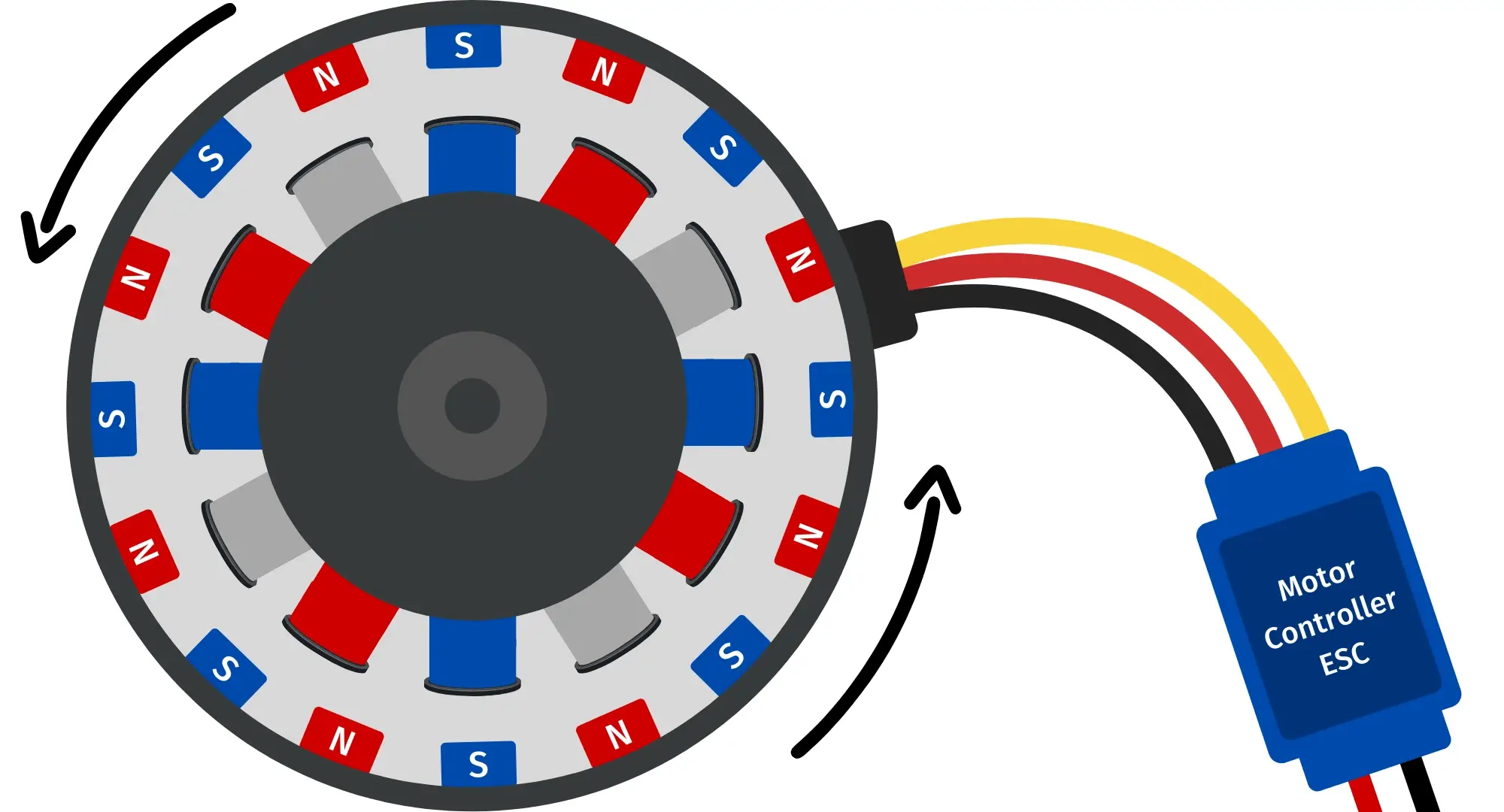
We are building an ESC
Just to be explicitly clear on how exactly this torque can vary, let’s take a few examples. Let’s look at a specific set of coils and a specific magnet on the rotor. In this case, the motor is spinning counter clockwise.
Example 1: The red (North polarity) permanent magnet on the rotor is attracted to blue S coil. And as our red permanent magnet approaches the blue S coil, the force of attraction begins to sharply increase because the force of magnetic pull is inversely proportional to distance squared. QED, torque sharply increases.

Example 2: Imagine the red permanent magnet is exactly over a coil. We do not want to ever have a permanent magnet directly over a coil it is attracted to, so we use the ESC to flip the polarity (making the N→S and S→N in the picture above). However, even when the rotor’s magnets being pushed away (or attracted) as they should, there will be an instant where a permanent magnet’s magnetic field is parallel to the direction of the magnetic field produced by the coil. By the following equation
\[F=qvBsin(\theta)\]We see that when $\theta$ is 0, $F$ is also equal to 0. We can thankfully rely on angular momentum to carry our rotor past this $\theta=0$ situation. We can also rely on small deviations in the positions of the permanent magnets (Imagine having the permanent magnets offset such that only one of them is ever at this $\theta=0$ condition, allowing the others to provide force as well).
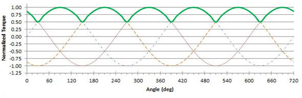
The result of those two examples, among a few other cases not described here, is an uneven torque as a function of $\theta$. An example of cogging torque is shown below.
We’ve now realized the need to have some function
\[\tau(I, \theta) = \tau_{sourced}\]To best achieve this, we can create a torque map. By attaching an IMU on an arm of a known length at a right angle to the output shaft of a motor, we can now measure angular acceleration.
It’s also worth noting that we specifically chose to not double-differentiate $\theta$ over time from an encoder because that method is incredibly sensitive to noise in $\theta$. Given that our maximum sweep of a realistic joint would never exceed 180$^{\circ}$, we would need an extremely accurate encoder.
With this IMU setup, a robust and fast current-sensing circuit for each phase, and an encoder, we can now effectively measure all our inputs to our ‘system’ (the motor) and it’s functional output.
With some neat EE tricks paired with some expensive mosfets and gate drivers, we can also modulate the current to modulate the torque. Given the high inductance and capacitance of BLCD motors due to their coils, modulating the power to the BLCD motor through PWM will give us a smooth-enough variable voltage on the coils.
We turn on the motor with a set current $I$, rotating approximately 180 degrees, and measure the angular acceleration. We generate $\dot{w}(\theta)$ at constant $I$, for several different $I$s
Doing this at different set $I$s, we begin to build a cogging torque map similar to one pictured above, except at different currents with different profiles. We see below an example, with the red plot clearly being at a lower set current.
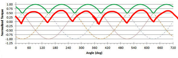
Modulating the current to build this map may actually be unnecessary, as the torque should be linearly related to the current input. The reason we can’t just use $\tau = k_t * I$ is because of the contours/curves that the cogging torque effect introduces. However, the ‘shape’ of that effect should depend only on the motor and not the current into that motor. In this case, that means only one calibration run.
Regardless, though, we are thus are able to build a map that where we can lookup the current torque our motor is producing as a function of current and angle.
\[\tau(I, \theta) = \tau_{sourced}\]This three-variable lookup map can be trivially modified to allow us to calculate the desired current given a desired torque and motor position.
\[I(\tau_{out}, \theta_{current}) = I_{out}\]The appropriate method of measuring $\theta$ is yet to be determined. An encoder is standard, but using an IMU or more accurate position sensor may be necessary.
2. Sensors and Mathematics of Assisted Motion
Expanding on our understanding of basic mechanics, we see that in a situation where the motor is sourcing a known torque, the overall acceleration of a limb is trivial. We sum that torque with the torque sourced by the human and divide by the moment of inertia in order to get the overall angular acceleration.
\[\dot{w} = \frac{(\tau_{sourced} + \tau_{human})}{m_{constant}}\]We use $m$ for the moment of inertia to avoid any confusion with using $I$ for current.
It’s worth noting, too, that there are some associated losses with any mechanical system. It is unclear whether or not these will be compensated for within an accurate control-loop. The equation is below.
\[\dot{w} = \frac{(\tau_{sourced} + \tau_{human} - \tau_{friction})}{m_{constant}}\]We’ve established a very simple equation to dictate the motion of a mass (or rod) when actuated around a point by two sources of torque. In essence, this directly translates to a simple model of an assisted human joint.
To be explicit, consider one’s elbow joint; one’s forearm is a rod actuated around the elbow by the torque applied by the bicep pulling on the joint ($\tau_{human}$). Introducing a motor to the joint provides the second source of torque ($\tau_{sourced}$).
Here is how we collect the relevant variables in this equation
$\dot{w}$ from the IMU sensing array
A specially-developed array of IMUs mounted rigidly to pertinent points on the body feed data into a simple set of filters and machine-learning model that deduces pose and the instantaneous angular acceleration on any limb.
$m_{constant}$ from a one-time calibration
We apply a very small and short known torque from the motor to a limb, and then measure the angular acceleration. We are able to remove the effect of gravity from this.
$\tau_{sourced}$ from our torque map
At any given moment, we are fully aware of the torque produced by the motor from our torque map.
3. Torques and Sensation of Assisted Motion
The physical sensation of weight is not necessarily the sensation of torque, but rather the sensation of the equivalent moment of inertia at a measured angular acceleration. Therefore, a natural sensation of assisted motion would literally be a reduction factor of the moment of inertia.
We establish the following equation to dictate the real moment of inertia, the perceived moment of inertia once assisted, and the factor by which things feel lighter.
\(m_{assisted} = (1-a) * m_{constant}\) where $a$ is the factor between 0% and 100% by which we reduce the weight
So a factor of $a=10%$ would mean that $m_{assisted} = 0.9 * m_{constant}$, which translates to your limb feeling 90% as heavy as it really is.
But back to the math. From the aforementioned equation
\[\dot{w}\checkmark = \frac{(\tau_{sourced}\checkmark + \tau_{human})}{m_{constant}\checkmark}\]we know the following:
- $\dot{w}$ from the IMU sensing array
- $m_{constant}$ from a one-time calibration
- $\tau_{sourced}$ from our torque map
The assumption of $m_{constant}$ being constant is a generous one - this essentially means that one could not pick an item up, thereby changing their forearm’s moment of inertia.
We are thus able to calculate the torque that the human is providing.
We can then use the following equation, which calculates the targeted angular acceleration if the human’s torque corresponds to $m_{assisted}$.
\[\dot{w}_{assisted} = \frac{\tau_{human}}{m_{desired}}\]To be explicitly clear, movement in the absence of any assistance is dictated by
\[\dot{w}_{actual} = \frac{\tau_{human}}{m_{constant}}\]So we want to provide assistive motion by reducing the perceived moment of inertia to $m_{assisted}$.
\[\dot{w}_{desired} = \frac{\tau_{human}}{m_{assisted}}\]This equation then means that we must make the angular acceleration of the body $\dot{w}_{desired}$
So we now have a target angular acceleration ($\dot{w}_{desired}$) that will result in an $a\%$ sensation of reduced weight
Expanding on simple mechanics, $\dot{w}_{desired}$ is some fraction of the torque needed
\[{\tau}_{needed} = w_{desired} \cdot m_{const} - \tau_{human}\] \[{\tau}_{needed} = w_{desired}\checkmark \cdot m_{constant\checkmark} - \tau_{human} \checkmark\]Again, it’s worth noting that there may be a significant bias term for bias torque\({\tau}_{needed} = w_{desired} \cdot m_{const} - \tau_{human} (+ \tau_{bias})\)
We take this full circle and then determine how to produce this needed torque ${\tau}_{needed}$ by utilizing our torque map
\[I(\tau_{out}\checkmark, \theta_{current}\checkmark) = I_{out}\]This current, $I_{out}$ may be impossible to reliably source to the motor, as temperature or back-emf may change the resistance, capacitance, and inductance. Electrically, at the board level, a tight PID control loop (with PWM duty cycle as the output, and target current as the input), may be necessary.
Summary
We build a static torque map by characterizing a BLDC motor \(\tau(I, \theta) = \tau_{sourced}\)
The angular acceleration of any system with mass about a hinge is governed by \(\dot{w} = \frac{(\tau)}{m_{constant}}\) where $m_{constant}$ denotes our moment of inertia, which itself must be measured
We then separate the total torque into the torque from the motor ($\tau_{motor}$) and the torque from the human ($\tau_{human}$). \(\dot{w} = \frac{(\tau)}{m_{constant}} = \frac{(\tau_{sourced} + \tau_{human})}{m_{constant}}\)